The Road not Tokenized — Ayush Baweja

I was working through Karpathy’s lecture on tokenizers and found an interesting asymmetry between the encoding and decoding phases of a tokenizer. To explore it, let’s take a toy vocabulary that maps token IDs to strings:

\begin{array}{ccl} \text{Token ID} & & \text{Decoded text} \\ \hline 0 & \longmapsto & \mathtt{a} \\ 1 & \longmapsto & \mathtt{b} \\ 2 & \longmapsto & \mathtt{c} \\ 3 & \longmapsto & \mathtt{ab} \\ 4 & \longmapsto & \mathtt{bc} \\ 5 & \longmapsto & \mathtt{abc} \end{array}

Now, suppose we want to encode the string abc. There are several valid ways to represent it:

Let $D$ denote the decoder and $\mathbin{\Vert}$ denote string concatenation. Then

\begin{aligned} D\bigl([5]\bigr) &= \mathtt{abc}, \\ D\bigl([3,2]\bigr) &= \mathtt{ab} \mathbin{\Vert} \mathtt{c} = \mathtt{abc}, \\ D\bigl([0,4]\bigr) &= \mathtt{a} \mathbin{\Vert} \mathtt{bc} = \mathtt{abc}, \\ D\bigl([0,1,2]\bigr) &= \mathtt{a} \mathbin{\Vert} \mathtt{b} \mathbin{\Vert} \mathtt{c} = \mathtt{abc}. \end{aligned}

These representations are all valid: decoding any of the four token sequences gives us the same string, abc. In practice, however, encoding abc with a particular deterministic tokenizer will always produce the same token sequence. That sequence is the tokenizer’s canonical encoding of abc.

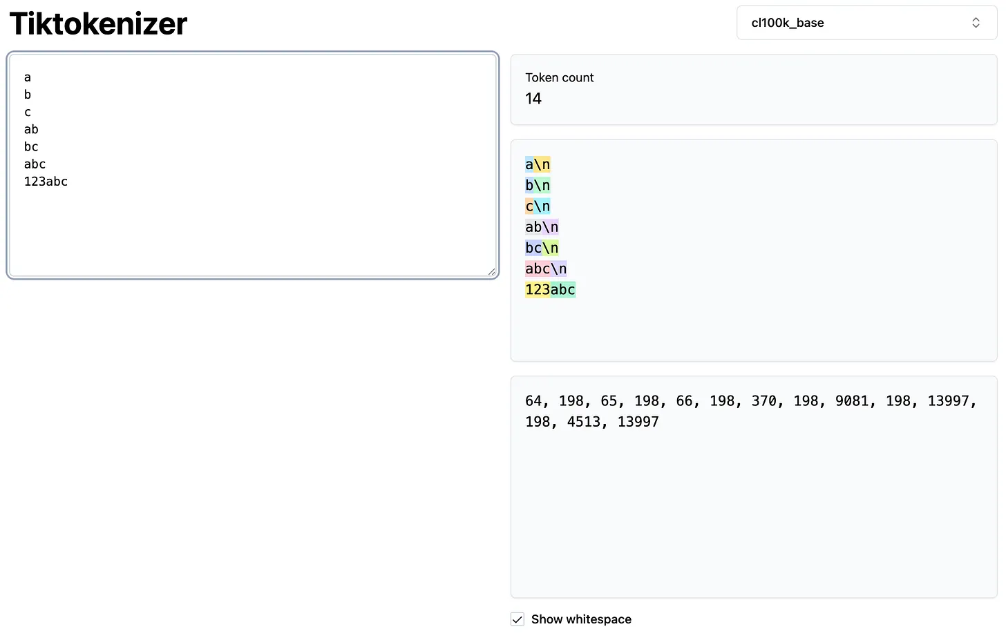
A tokenizer treating abc as one token within the string 123abc — Each letter and two-letter combination maps to a token on its own, but in the string `123abc`, `abc` is treated as a single token.

An interesting way to visualize the possible encodings is as a graph:

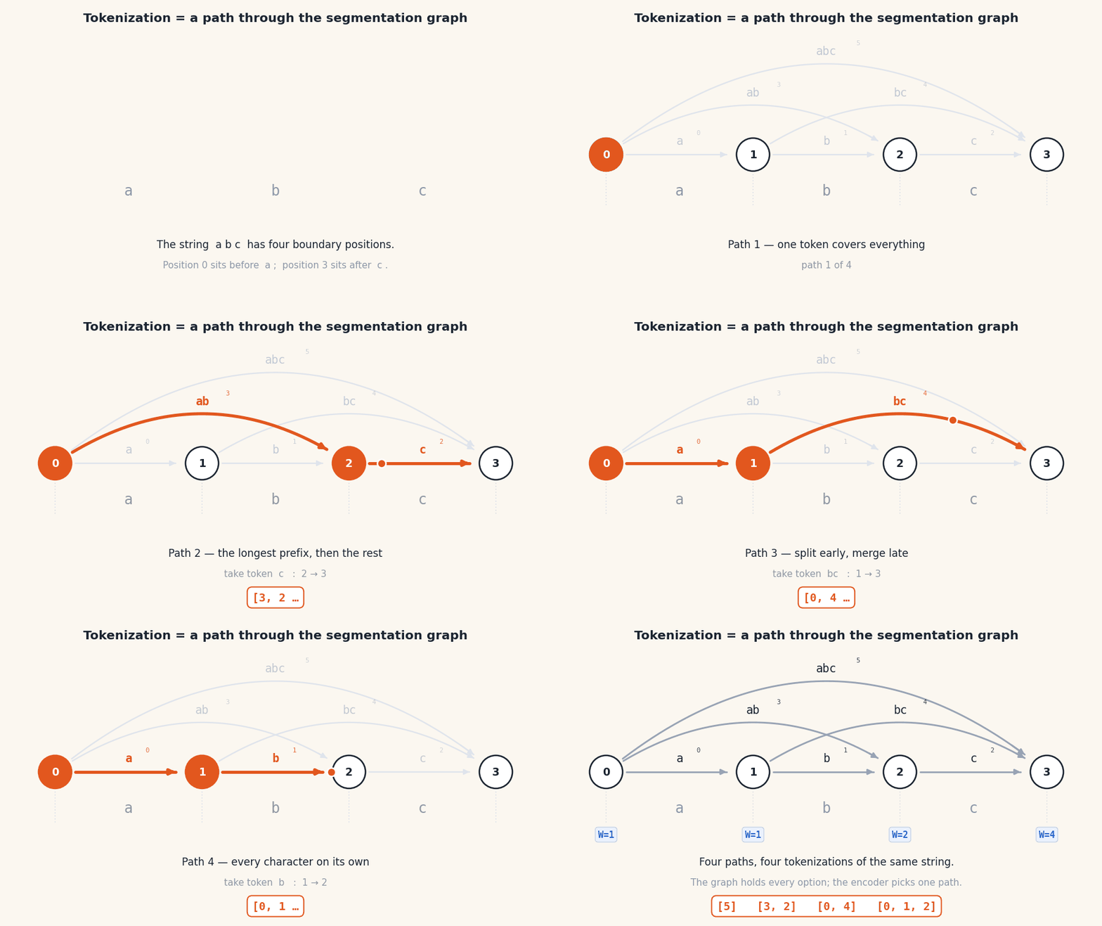
Animation showing the four paths through the tokenization graph for abc — Every path from the start of the string to its end is a valid tokenization.

Start by placing a node at every character boundary. Each edge represents a token in our vocabulary, and any valid encoding of abc is a path from node 0 to node 3 that neither overlaps tokens nor leaves gaps. The vocabulary determines the possible edges; the encoder decides which path to take.

Working backwards, the number of ways to reach the final position is the sum of the numbers of unique ways to reach every position with an edge into the final node. Solving this recursively for our toy vocabulary gives us four paths, as expected.

So the asymmetry is this: in a lossless tokenizer, decoding an encoded string returns the original string, but re-encoding a decoded token sequence may not return the original token sequence. Formally,

\begin{aligned} D\bigl(E(s)\bigr) &= s && \text{for every representable string } s, \\ E\bigl(D(z)\bigr) &\neq z && \text{in general.} \end{aligned}

For example, let $E$ be the encoder and take the non-canonical token sequence $z = [0,1,2]$ :

\begin{aligned} D(z) &= \mathtt{abc}, \\ E\bigl(D(z)\bigr) &= E(\mathtt{abc}) = [5] \neq [0,1,2] = z. \end{aligned}

The example exposes a distinction that is normally hidden by a standard deterministic encoder. A string $s$ does not necessarily correspond to a single token sequence; it corresponds to the set

\mathcal{T}(s) = \left\{ z \in \mathcal{V}^{*} \;\middle|\; D(z) = s \right\},

where $\mathcal{V}^{*}$ is the set of all finite sequences over the token vocabulary. The encoder chooses one representative $E(s) \in \mathcal{T}(s)$ from that set.

To select a canonical encoding, the encoding function has to follow a rule. Byte Pair Encoding (BPE) applies a ranked list of merges learned from the frequency of adjacent token pairs in the tokenizer’s training corpus.

A note on length: BPE does not guarantee the shortest possible token sequence for a string. It follows its ranked merge rules to produce the final encoding. Other tokenizers could use different rules, such as always selecting the longest matching vocabulary element or explicitly searching for the shortest token sequence.

Does the Model Care?

This realization surfaced a few related questions.

An autoregressive language model assigns probabilities to token sequences. But if multiple token sequences decode to the same string, then the probability of that string is, in principle, the sum of the probabilities of all those tokenizations. Enumerating them quickly becomes computationally expensive, so using only the probability of the canonical tokenization seems like a justified compromise. Are we missing important information by doing that? In the same vein, does a model treat different tokenizations of the same string differently?

The paper Where Is the Signal in Tokenization Space? explores whether non-canonical tokenizations of a string provide any additional signal beyond its canonical tokenization. Instead of just the canonical tokenization, they consider the most likely tokenization and a marginal probability over all possible tokenizations.

When attempting to find the most likely tokenization, the authors of the paper set the probability of the canonical tokenization as a baseline and search for paths with a higher probability, pruning those paths with a partial probability below the canonical. Under a time limit, despite exponential growth in tokenization paths as the string length increases, the authors did not find any tokenization that beat the canonical baseline.

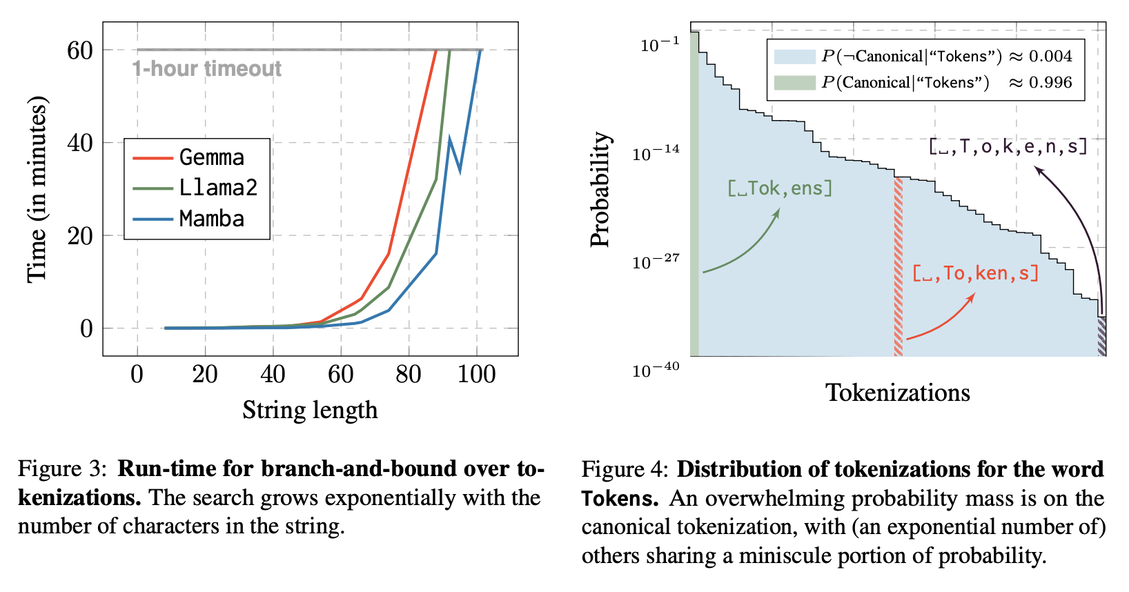
Plots of tokenization search time and probability mass across tokenizations — Branch-and-bound search time grows rapidly with string length (left), while nearly all probability mass for `Tokens` lies on its canonical tokenization (right).

The marginal probability (the sum of the probabilities of every possible tokenization) of short strings was found to converge to the canonical tokenization’s probability. To estimate the marginal probability of longer strings, the authors use importance sampling. Here, they add a one-step lookahead constraint and mask out tokens that would prevent spelling the target string. This is done until the complete string is produced and then they sample a tokenization. Again, despite this method, the authors find that as the samples increase, the marginal converges close to the canonical probability. Thus, the canonical tokenization has the bulk of the probability mass.

To test whether there is any signal in these low-probability, non-canonical tokenizations, the authors draw a number of non-canonical tokenizations of the answers for multiple choice questions while keeping the questions in their standard tokenizations. The authors estimate each answer’s marginal using k sampled tokenizations, tune the sample count k on a 1000-example validation set and apply that k to the test set. The test set includes multiple-choice benchmarks such as HellaSwag, SocialIQA and OpenBookQA across several models and find modest improvement in accuracy. Using a weighted mix of canonical and non-canonical probabilities also led to accuracy improvements, leading the authors to conclude clear signal.

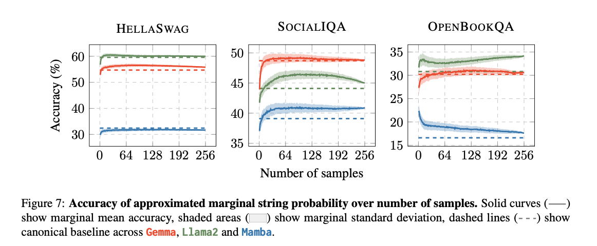
The hypothesis the paper is seemingly drawing towards is that ignoring the non-canonical tokenizations is throwing away meaningful signal; the true probability of a string is not equivalent to the canonical tokenization probability. As seen from the graph, as the number of samples increased, performance tended to return to the canonical baseline. With more samples, the estimate of the true marginal probability gets more accurate and so this decrease in performance contradicts the idea that there is signal there. The true marginal is essentially canonical as the authors found, then as you estimate the marginal better, you recover the canonical score. The tuned classifier improved accuracy here and the weighted experiment also improved accuracy, so there is some evidence of information but no clear reason why.

The authors of Broken Tokens? Your Language Model Can Secretly Handle Non-Canonical Tokenizations take this question further by asking whether the model really understands these alternate tokenizations in the input. To start, they experiment to see if models can retain performance during inference when provided with random or character-level encodings during inference. Reinforcing the robustness of these models, they find that instruction tuned models retain 90%+ performance compared to canonical tokenizations on their benchmarks.

Establishing that the models are capable of retaining performance, the authors of this paper also test whether these non-canonical tokens can improve performance on various tasks: character counting, acronyms, code description, and arithmetic. This alludes to the strawberry problem where LLMs struggled to count the occurences of the letter ‘r’ in ‘strawberry’. Testing shows that the training tokenization is often not optimal for some tasks; large improvements were seen in code description and arithmetic by using alternative tokenizations.

As noted earlier, these improvements were seen in instruct models, which leads to another research question. At what point in the post-training do models develop robustness to non-canonical tokenizations? To identify the source, testing was done with the base, SFT, DPO and instruct models again based on spelling, grammatical correctness and the preference of an LLM Judge system between the responses to a canonical and non-canonical prompt.

The base models clearly struggle with the task but do represent understanding of the context. The bulk of the improvement comes from the SFT stage.

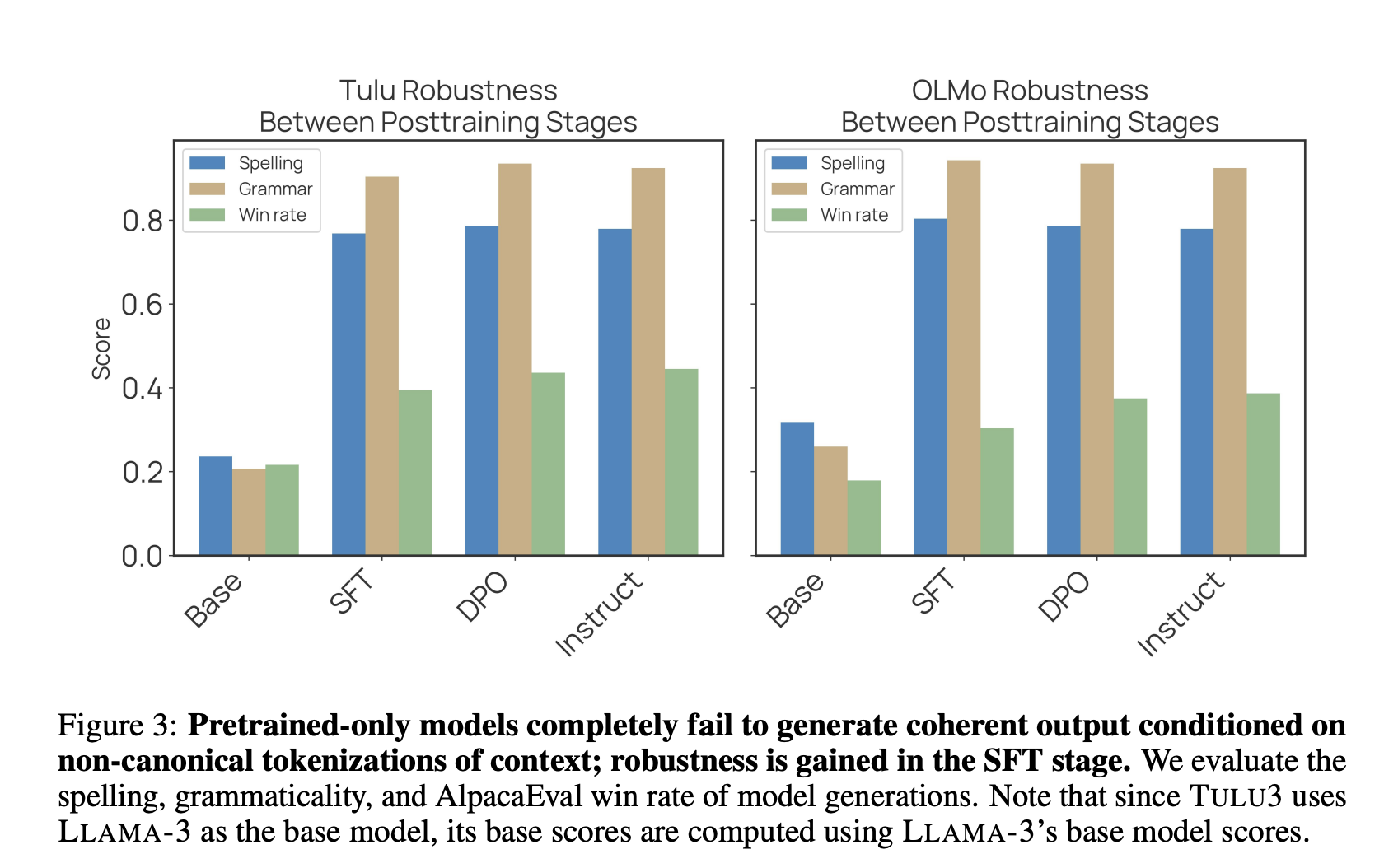
Further ablation studies on the SFT stage show that the chat template tags (separation of question and response) and the keeping the format more like question and response instead of continuation (even with tags) are key to robustness. The authors conclude that token boundaries can act as an inference-time representation control, producing large gains when they align with task structure and that this robustness arises as a an artifact of post training a base model.

Conclusion

The initial asymmetry brought up several fascinating research results:

A string can have multiple valid tokenizations, even though a deterministic tokenizer picks one path as canonical.
Canonical tokenization usually captures nearly all probability mass.
Experimental results show that these low-probability alternatives can still contain task-relevant representations.
Instruction tuning in particular may lead to model robustness to non-canonical tokenizations.